# 文本检测FCENet
论文:Fourier Contour Embedding for Arbitrary-Shaped Text Detection (opens new window)
# 1.简介
这篇文章是华南理工大学的Yiqin Zhu在2021年04月份发表的有关OCR中做文本检测的工作。一般OCR工作分两步,一步是对文本区域进行检测,先得到文本区域,然后再将检测的文本区域转化成文本。
文本检测的复杂性在于文本区域的步规则性和多样性,常用的在图像空间域做文本检测方法有掩码,像素的笛卡尔或极坐标坐标轮廓点。使用掩码来做需要对图像进行像素级分类后处理时间较长,使用轮廓像素点在处理弯曲文本区域时略显无力。文本检测的方法可粗略的分成基于分割的方法和基于回归的方法。
作者提出的方法在频域对文本区域做检测,使用Fourier Contour Embedding(FCE)方法来表示任意行状的文本轮廓。FCENet模型中使用了骨干网络(backbone),特征金字塔往略(Feature Pyramid Network),带傅里叶逆变换(Inverse Fourier Transform,IFT)的后处理,和非极大值抑制。FCENet最大的创新在于其使用神经网络直接对文本轮廓点的傅里叶变换做预测,然后再使用IFT求得最后的文本轮廓。
使用
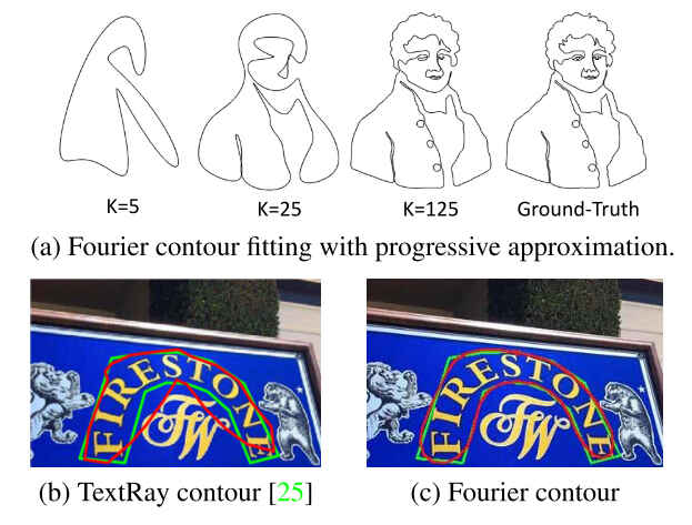
从上图(a)中可以看到,当TextRay和FCENet来做文本检测所得到的结果,绿色的是真实的文本轮廓线,可以看到对弯曲的文本,FCENet检测效果更好。
# 2.主要工作
# 2.1 傅里叶轮廓嵌入(Fourier Contour Embedding)
对于图像中使用像素坐标点
其中
到这里轮廓线上点的坐标
若已经知道
其中,
图像中的轮廓曲线一般很难得到其函数表示
利用欧拉公式,
当
傅里叶轮廓嵌入算法(Fourier Contour Embedding)算法分两步,第一步是对轮廓进行采样离散化,譬如在轮廓上均匀采样400个点FCE算法支持更多的数据集合,因为不同数据集标注的文本区域轮廓点的数目并不一样。第二步就是进行傅里叶变换和反变换,求目标值和文本区域的检测框坐标。
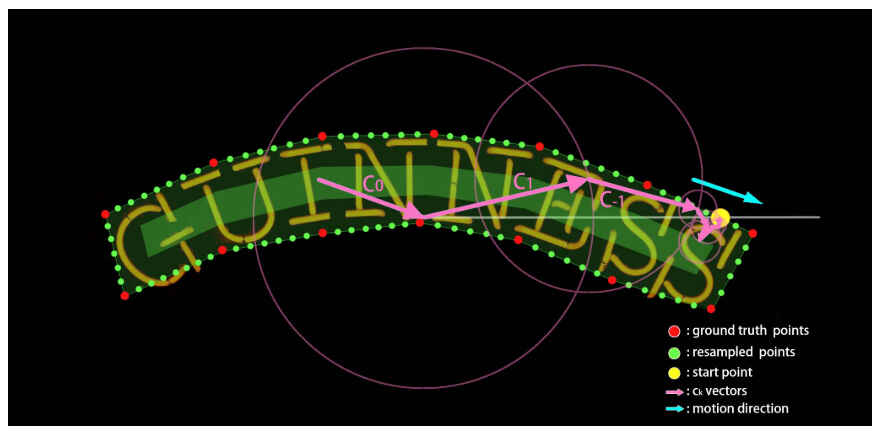
采样策略:
- 采样起始点
- 采样方向,顺时针
- 匀速,每两个采样点的距离相同
可以通过一段代码来看:
import numpy as np
import matplotlib.pyplot as plt

x = np.array(list(range(10, 210, 10)))
y = np.array([10]*len(x))
x = x[:,None]
y = y[:,None]
pnts = np.concatenate((x,y), axis=-1)

y = np.array(list(range(20, 120, 10)))
x = np.array([200]*len(y))
x[5] = 220
x[6] = 214
x[7] = 207
x[8] = 203

x = x[:,None]
y = y[:,None]
tmp_pnts = np.concatenate((x,y), axis=-1)
pnts = np.vstack((pnts, tmp_pnts))

x = np.array(list(range(190, 0, -10)))
y = np.array([110]*len(x))
x = x[:,None]
y = y[:,None]
tmp_pnts = np.concatenate((x,y), axis=-1)
pnts = np.vstack((pnts, tmp_pnts))

y = np.array(list(range(100, 10, -10)))
x = np.array([10]*len(y))
x = x[:,None]
y = y[:,None]
tmp_pnts = np.concatenate((x,y), axis=-1)
pnts = np.vstack((pnts, tmp_pnts))

pt1 = pnts[:24,:]
pt2 = pnts[24:,:]
pts = np.vstack((pt2, pt1))

complex_pts = pts[:, 0] + pts[:, 1]*1j
ft_pts = np.fft.fft(complex_pts)

approx_ft_pts = np.zeros_like(ft_pts)
# 信号主要由高频和低频组成,中间频率所占很少
approx_ft_pts[:6] = ft_pts[:6] # 低频信号恢复大致轮廓
approx_ft_pts[-5:] = ft_pts[-5:] #高频信号恢复准确轮廓
appox_pts = np.fft.ifft(approx_ft_pts)

# help(plt.plot)
plt.figure(num=1, figsize=(4.5,3), dpi=200)
x = pts[:, 0]
y = pts[:, 1]
plt.plot(x,y,'g-', label='ground truth', linewidth=1 )
x = [e.real for e in appox_pts]
y = [e.imag for e in appox_pts]

plt.plot(x,y,'r-', label='approx truth', linewidth=1 )
plt.legend()
plt.show()

上图中,绿色的表示实际形状,红色的表示经傅里叶变换和反变换后,只保留
# 2.2 FCE模型
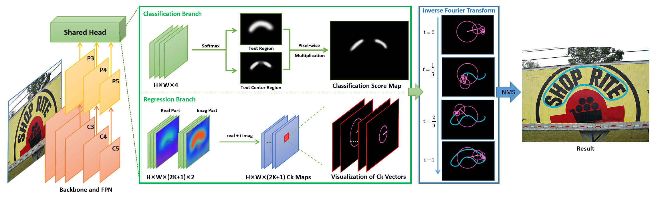
FCENet的结构同常规的检测模型,其backbone由使用可变形卷积DCN的ResNet50组成,FPN用来提取多尺度的特征,检测头使用以上介绍的傅里叶方法实现。
如上图,检测头由分类和回归两个分支组成,分类分支中,输出的结果通道数是4,前两个通道表示的是每个像素是否是文本区域(Text Region,TR)的概率,后两个通道表示的是每个像素是否是文本中心区域(Text Center Region)的概率,分类分支相当于是分割得到文本区域,然后求文本区域的轮廓中心。
回归分支的通道数
# 3.代码实现
见mmocr: mmocr/models/textdet/postprocessors/fce_postprocessor.py (opens new window)
class FCEPostprocessor(BaseTextDetPostProcessor):
     def __init__(self, **args):
          ...
     def _get_text_instances_single(self, pred_result: Dict, scale: int):
          """Get text instance predictions from one feature level.

          Args:
               pred_result (dict): A dict with keys of ``cls_res``, ``reg_res``
                    corresponding to the classification result and regression
                    result computed from the input tensor with the same index.
                    They have the shapes of :math:`(1, C_{cls,i}, H_i, W_i)` and
                    :math:`(1, C_{out,i}, H_i, W_i)`.
               scale (int): Scale of current feature map which equals to
                    img_size / feat_size.

          Returns:
               result_polys (list[ndarray]): A list of polygons after postprocess.
               result_scores (list[ndarray]): A list of scores after postprocess.
          """

          cls_pred = pred_result['cls_res']
          tr_pred = cls_pred[0:2].softmax(dim=0).data.cpu().numpy()
          tcl_pred = cls_pred[2:].softmax(dim=0).data.cpu().numpy()

          reg_pred = pred_result['reg_res'].permute(1, 2, 0).data.cpu().numpy()
          x_pred = reg_pred[:, :, :2 * self.fourier_degree + 1]
          y_pred = reg_pred[:, :, 2 * self.fourier_degree + 1:]

          score_pred = (tr_pred[1]**self.alpha) * (tcl_pred[1]**self.beta)
          tr_pred_mask = (score_pred) > self.score_thr
          tr_mask = fill_hole(tr_pred_mask)

          tr_contours, _ = cv2.findContours(
               tr_mask.astype(np.uint8), cv2.RETR_TREE,
               cv2.CHAIN_APPROX_SIMPLE)  # opencv4

          mask = np.zeros_like(tr_mask)

          result_polys = []
          result_scores = []
          for cont in tr_contours:
               deal_map = mask.copy().astype(np.int8)
               cv2.drawContours(deal_map, [cont], -1, 1, -1)

               score_map = score_pred * deal_map
               score_mask = score_map > 0
               xy_text = np.argwhere(score_mask)
               dxy = xy_text[:, 1] + xy_text[:, 0] * 1j

               x, y = x_pred[score_mask], y_pred[score_mask]
               c = x + y * 1j
               c[:, self.fourier_degree] = c[:, self.fourier_degree] + dxy
               c *= scale

               polygons = self._fourier2poly(c, self.num_reconstr_points)
               scores = score_map[score_mask].reshape(-1, 1).tolist()
               polygons, scores = self.poly_nms(polygons, scores, self.nms_thr)
               result_polys += polygons
               result_scores += scores

          result_polys, result_scores = self.poly_nms(result_polys,
                                                       result_scores,
                                                       self.nms_thr)

          if self.text_repr_type == 'quad':
               new_polys = []
               for poly in result_polys:
                    poly = np.array(poly).reshape(-1, 2).astype(np.float32)
                    points = cv2.boxPoints(cv2.minAreaRect(poly))
                    points = np.int0(points)
                    new_polys.append(points.reshape(-1))

               return new_polys, result_scores
          return result_polys, result_scores

     def _fourier2poly(self,
                         fourier_coeff: np.ndarray,
                         num_reconstr_points: int = 50):
          """ Inverse Fourier transform
               Args:
                    fourier_coeff (ndarray): Fourier coefficients shaped (n, 2k+1),
                    with n and k being candidates number and Fourier degree
                    respectively.
                    num_reconstr_points (int): Number of reconstructed polygon
                    points. Defaults to 50.

               Returns:
                    List[ndarray]: The reconstructed polygons.
               """

          a = np.zeros((len(fourier_coeff), num_reconstr_points),
                         dtype='complex')
          k = (len(fourier_coeff[0]) - 1) // 2

          a[:, 0:k + 1] = fourier_coeff[:, k:]
          a[:, -k:] = fourier_coeff[:, :k]

          poly_complex = ifft(a) * num_reconstr_points
          polygon = np.zeros((len(fourier_coeff), num_reconstr_points, 2))
          polygon[:, :, 0] = poly_complex.real
          polygon[:, :, 1] = poly_complex.imag
          return polygon.astype('int32').reshape(
               (len(fourier_coeff), -1)).tolist()